Drone-based crop damage assessment: measured, not estimated
For a 9.43-hectare maize field we produced defensible figures from drone data: 0.69% of the area damaged, 5.51% unused, average plant height 2.1 metres, stand density around 29,600 plants per hectare – plus the growth stage at the time of capture.
The situation
Damage in the field is traditionally assessed by walking it and judging by eye, for instance after an extreme weather event. The result is an estimate, and estimates are unreliable at small percentages.
Yet a good deal hangs on it. Insurance claims, reseeding decisions and yield forecasts all depend on the damage assessment. Anyone who cannot distinguish one percent from five is deciding on a basis that does not deserve the name – and at that scale, the difference between an estimate and a measurement is the difference between a supposition and evidence.
The data
A maize field of roughly 9.43 hectares, captured by drone. The data came in two forms: raw imagery with four spectral bands, and a LAS point cloud.
Processing ran on a basemap in the WGS 1984 Web Mercator projection with vertical units in metres. Only that yields a georeferenced, integrated spatial dataset – the precondition for a measured area also being attributable to a location in the field.
Challenges
Correction before analysis. The raw images were first stitched into an orthomosaic. Ahead of that came the step that determines whether any later figure is defensible: radiometric correction. Measured brightness values of individual pixels, band-to-band errors, and geometric and panoramic distortions from the capture process all had to be compensated.
Without that step, a model classifies differences in illumination and capture geometry as damage. The percentages would look every bit as precise – and would be wrong. This is the unspectacular part of such projects, and the part on which they stand or fall.
Approach
Compare supervised against unsupervised. We applied both classification approaches to the orthomosaic. The unsupervised approach shows what structures the data yields on its own; the supervised one tests the categories defined by domain knowledge. Only together do they give confidence that an area identified really is damaged area.
Pixel-wise classification by spectral properties. The trained algorithm assigns every pixel of the orthomosaic to a class based on its spectral signature. That produces the delineated damaged and unused areas from which area shares can be calculated.
Derive height from the point cloud. From the LAS dataset we generated a digital elevation model and a digital surface model. The difference between the two yields plant height – information that cannot be obtained from the imagery alone, and which brings the third dimension into the assessment.
Growth stage via the vegetation index. An NDVI estimate on the raster images, together with careful photointerpretation, established the growth stage of the maize. That is decisive for interpreting the result: the same damage share means something entirely different for yield depending on development stage.
Outcome
For the 9.43-hectare field, the analysis produced:
- 5.51% of the area unused
- 0.69% of the area classified as damaged
- 2.1 m average plant height
- around 29,600 plants per hectare stand density
- maize in the reproductive growth phase at the time of capture
The ratio is the notable part: the unused area is eight times the size of the damaged area. That is a yield problem with nothing to do with the weather event, and one that a field walk would not register as such – because nobody adds up unused patches.
Transferability
The sequence – radiometrically correct raw data, consolidate it into a georeferenced dataset, classify it, add the third dimension from a point cloud, and report the result as an area share – reaches beyond crop damage: infestation detection, stand density, growth monitoring, area accounting. Wherever an area has to be quantified rather than merely described.
Today
The capture side has changed most: RTK-enabled drones with multispectral sensors now deliver georeferenced data at an accuracy that used to require ground control points. In classification, deep learning methods replace purely pixel-wise spectral assignment – they take texture and surroundings into account and are consequently more robust to differences in illumination. We now determine plant counts through object detection rather than density estimation. Point clouds are processed with PDAL in cloud-native formats, raster data as Cloud-Optimized GeoTIFF with STAC cataloguing, which is what makes analysis across many areas and time points practical in the first place. And to scale from one field to a region we combine drone imagery with satellite time series: the drone for accuracy, Sentinel data for extent and progression.
Last updated: 30 July 2026